Interpolation

What is Interpolation?

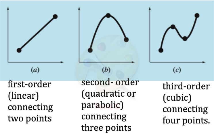
Interpolation is a method of estimating unknown data points that lie between known data points. Think of it as “connecting the dots” with a mathematical function.

Key Points:

• Constructs new data points based on a discrete set of known data points
• Creates a function that passes through ALL given data points exactly
• Used to estimate values between the given data points

Important Theorem

Weierstrass Approximation Theorem: For any continuous function on a closed interval, there exists a polynomial that can approximate it as closely as desired.

Key Result: For data points, there is exactly one polynomial of degree that passes through all the points.

---

Newton’s Divided-Difference Method

The Newton Form

For data points, the interpolating polynomial has the form:

Finding the Coefficients

Step 1: Set

Step 2: Set

Step 3: Set

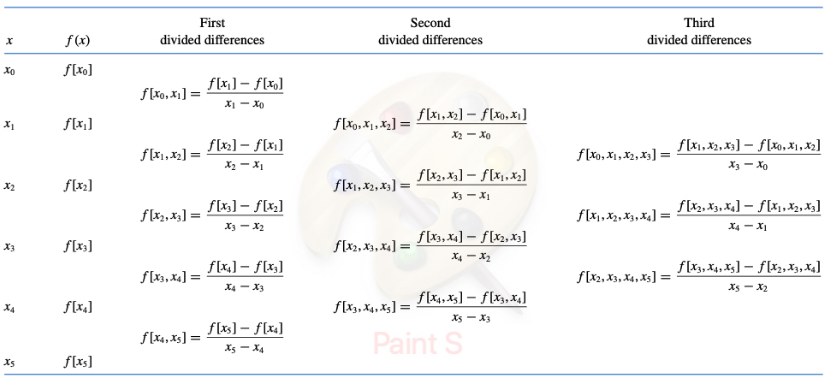
Divided Difference Notation

Zeroth divided difference:

First divided difference:

Second divided difference:

General -th divided difference:

Newton’s Divided Difference Formula

The coefficients are:

Final Newton Form:

---

4.1.2 Lagrange Interpolating Polynomials

The Lagrange Form

The same interpolating polynomial can be written as:

where the Lagrange basis polynomials are:

Examples of Lagrange Polynomials

For (Linear interpolation):

For (Quadratic interpolation):

Example: Current in Wire

Given data:

t	0	0.1250	0.2500	0.3750	0.5000
i	0	6.24	7.75	4.85	0.0000

Problem: Find at

---

Errors in Interpolating Polynomials

Error Formula

For a function and distinct points in :

where is some unknown point in the interval.

Error Estimation

Theoretical error:

Practical error estimation (using additional data point):

---

Least Squares Approximation

When to Use Least Squares

Unlike interpolation (which passes through all points exactly), least squares finds the “best fit” curve that minimizes the overall error when:

• Data contains measurement errors
• We want a simpler model than exact interpolation
• We have more data points than we want polynomial degree

The Least Squares Principle

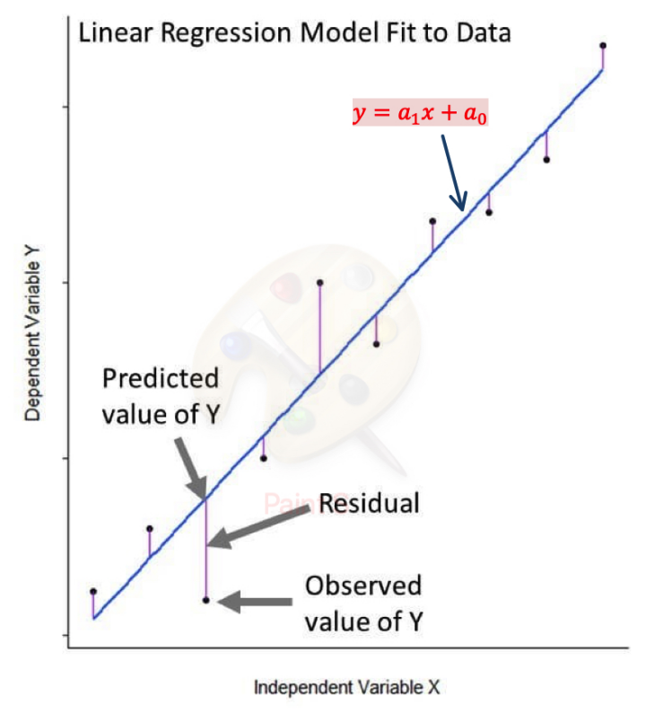
Residual (error):

Objective: Minimize the sum of squared errors:

---

Linear Regression

The Linear Model

Find the best line:

Sum of squared errors:

Finding the Coefficients

To minimize , we need:

This gives us the normal equations:

Example: River Flow Prediction

Given data:

Precipitation (cm)	88.9	108.5	104.1	139.7	127.0	94.0	116.8	99.1
Flow (m³/s)	14.6	16.7	15.3	23.2	19.5	16.1	18.1	16.6

Problem: Predict annual water flow for 120 cm precipitation.

---

Polynomial Regression

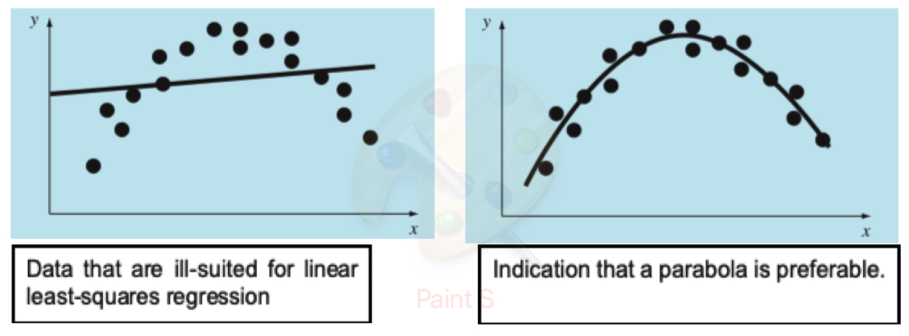
When Linear Isn’t Enough

Sometimes data follows a curved pattern that a straight line can’t capture well.

The Polynomial Model

Fit a polynomial of degree :

General Method

Minimize:

Normal equations: For :

This creates a system of equations in unknowns.

Example: Population Growth

Given data:

t (years)	0	5	10	15	20
p (population)	100	200	450	950	2000

Problem: Use 3rd-order polynomial regression to predict population at years.

---

Summary

Key Differences

Method	Purpose	Passes Through Points?	Best For
Interpolation	Exact fit	Yes, all points	Clean data, need exact values
Least Squares	Best approximation	No, minimizes error	Noisy data, want simple model

When to Use Each Method

Use Interpolation when:

• Data is precise and error-free
• You need exact values at given points
• You want to estimate between known points

Use Least Squares when:

• Data contains measurement errors
• You want a simpler model than exact interpolation
• You have more data points than desired polynomial degree
• You want to predict trends and patterns